Errors and Data Filtering#
All data fields contain corresponding errors, which should be used to correctly interpret the significance of the data. Additionally, there are some filters based on data quality metrics in the data files that are recommended for most scientific applications.
import h5py
import os
import urllib.request
import numpy as np
import matplotlib.pyplot as plt
Download files that will be used in this tutorial.
# Download the file that we need to run these examples
filename = 'data/20200207.001_lp_5min-fitcal.h5'

if not os.path.exists(filename):
    url='https://data.amisr.com/database/dbase_site_media/PFISR/Experiments/20200207.001/DataFiles/20200207.001_lp_5min-fitcal.h5'

    print('Downloading data file...')
    urllib.request.urlretrieve(url, filename)

    print('...Done!')
Error Fields#
Electron density errors are found in the FittedParams/dNe array. Errors for all other parameters can be found in the FittedParams/Errors array, which is constructed analogously to the Fits array.
with h5py.File(filename, 'r') as h5:

    rng = h5['FittedParams/Range'][:]
    Ne = h5['FittedParams/Ne'][:]
    utime = h5['Time/UnixTime'][:,0]

    # Read in all error arrays
    dNe = h5['FittedParams/dNe'][:]
    dTi = h5['FittedParams/Errors'][:,:,:,0,1]
    dTe = h5['FittedParams/Errors'][:,:,:,-1,1]
    dVlos = h5['FittedParams/Errors'][:,:,:,0,3]

time = utime.astype('datetime64[s]')
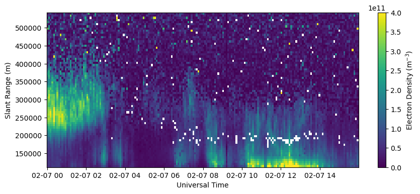
Plot RTI of electron density in beam 0.
fig = plt.figure(figsize=(10,4))
ax = fig.add_subplot(111)
c = ax.pcolormesh(time, rng[0,np.isfinite(rng[0,:])], Ne[:,0,np.isfinite(rng[0,:])].T, vmin=0., vmax=4.e11)
ax.set_xlabel('Universal Time')
ax.set_ylabel('Slant Range (m)')
fig.colorbar(c, label=r'Electron Density (m$^{-3}$)')
<matplotlib.colorbar.Colorbar at 0x7fe28e41abf0>

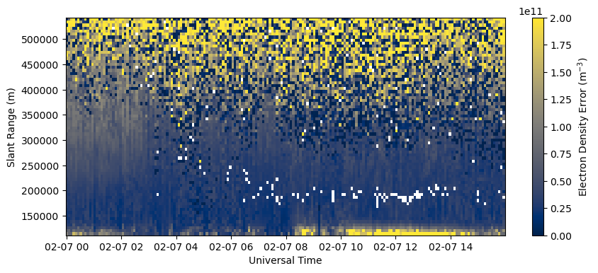
Plot RTI of electron density error in beam 0.
fig = plt.figure(figsize=(10,4))
ax = fig.add_subplot(111)
c = ax.pcolormesh(time, rng[0,np.isfinite(rng[0,:])], dNe[:,0,np.isfinite(rng[0,:])].T, vmin=0., vmax=2.e11, cmap='cividis')
ax.set_xlabel('Universal Time')
ax.set_ylabel('Slant Range (m)')
fig.colorbar(c, label=r'Electron Density Error (m$^{-3}$)')
<matplotlib.colorbar.Colorbar at 0x7fe2860fb430>

Note how the errors increase substantially at longer ranges where the radar is less sensitive.
Data Quality Filtering#
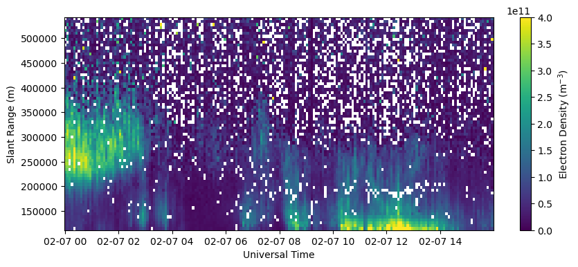
AMISR data files contain two useful data quality parameters, both in the FittedParams/FitInfo group. The first is fitcode, which is an indication of whether or not the fitting software used to process the raw data successfully converged. A parameter should only be used if fitcode has a value of 1, 2, 3, or 4. The second is chi2, which is the \(\chi^2\) goodness-of-fit parameter. This is expected to be somewhere around 1 because of statistical variability. If chi2 is substantially greater than 1, it indicates this was a very poor fit and the model is not a good match for the data, and therefor the output parameter should not be used. If chi2 is substantially less than 1, it is also suspect because it suggests very little variance in the data, which is not characteristic of incoherent scatter. It is possible that this point is instead a coherent echo off a hard-target (such as a metallic satellite in the radar’s beam), which erroneously looks like a very high density value with a very low error. A reasonable value for chi2 is between 0.1 - 10 for most situations.
with h5py.File(filename, 'r') as h5:
    fitcode = h5['FittedParams/FitInfo/fitcode'][:]
    chi2 = h5['FittedParams/FitInfo/chi2'][:]

print(Ne.shape, fitcode.shape, chi2.shape)
(188, 11, 74) (188, 11, 74) (188, 11, 74)
Note that the fitcode and chi2 arrays have the same shape as all the other data arrays. These data quality parameters can be applied to all data arrays equally - there are not separate data quality parameters for each of the four main data parameter.
Plot electron data filtered based on data quality parameters.
bad_data = np.logical_or(~np.isin(fitcode, [1,2,3,4]), np.logical_or(chi2<0.1, chi2>10.))
Ne_filt = Ne.copy()
Ne_filt[bad_data] = np.nan

fig = plt.figure(figsize=(10,4))
ax = fig.add_subplot(111)
c = ax.pcolormesh(time, rng[0,np.isfinite(rng[0,:])], Ne_filt[:,0,np.isfinite(rng[0,:])].T, vmin=0., vmax=4.e11)
ax.set_xlabel('Universal Time')
ax.set_ylabel('Slant Range (m)')
fig.colorbar(c, label=r'Electron Density (m$^{-3}$)')
<matplotlib.colorbar.Colorbar at 0x7fe27ee1ff70>

Plot electron density filtered by data quality parameters and where the density error is greater than the density (relative error greater than 1).
bad_data = np.logical_or(~np.isin(fitcode, [1,2,3,4]), np.logical_or(chi2<0.1, chi2>10.), Ne<dNe)
Ne_filt = Ne.copy()
Ne_filt[bad_data] = np.nan

fig = plt.figure(figsize=(10,4))
ax = fig.add_subplot(111)
c = ax.pcolormesh(time, rng[0,np.isfinite(rng[0,:])], Ne_filt[:,0,np.isfinite(rng[0,:])].T, vmin=0., vmax=4.e11)
ax.set_xlabel('Universal Time')
ax.set_ylabel('Slant Range (m)')
fig.colorbar(c, label=r'Electron Density (m$^{-3}$)')
<matplotlib.colorbar.Colorbar at 0x7fe27eb73130>


