Resolved Vector Velocities - “New” Version#
This tutorial covers how to read in, plot, and work with the new output vector velocities data product.
WIP
This page is currently a work in progress, meaning it likely has incomplete explanations and some non-functional code/links/ect. Please be patient!
If you think you can help, please consider contributing.
%matplotlib inline
import datetime
import matplotlib.pyplot as plt
import matplotlib.gridspec as gridspec
import matplotlib.dates as mdates
import re
import h5py
import numpy as np
from apexpy import Apex
import pymap3d as pm
import cartopy.crs as ccrs
A module that was compiled using NumPy 1.x cannot be run in
NumPy 2.0.0 as it may crash. To support both 1.x and 2.x
versions of NumPy, modules must be compiled with NumPy 2.0.
Some module may need to rebuild instead e.g. with 'pybind11>=2.12'.

If you are a user of the module, the easiest solution will be to
downgrade to 'numpy<2' or try to upgrade the affected module.
We expect that some modules will need time to support NumPy 2.

Traceback (most recent call last):  File "/usr/share/miniconda/envs/buildjupyterbook/lib/python3.10/runpy.py", line 196, in _run_module_as_main
    return _run_code(code, main_globals, None,
  File "/usr/share/miniconda/envs/buildjupyterbook/lib/python3.10/runpy.py", line 86, in _run_code
    exec(code, run_globals)
  File "/usr/share/miniconda/envs/buildjupyterbook/lib/python3.10/site-packages/ipykernel_launcher.py", line 18, in <module>
    app.launch_new_instance()
  File "/usr/share/miniconda/envs/buildjupyterbook/lib/python3.10/site-packages/traitlets/config/application.py", line 1075, in launch_instance
    app.start()
  File "/usr/share/miniconda/envs/buildjupyterbook/lib/python3.10/site-packages/ipykernel/kernelapp.py", line 739, in start
    self.io_loop.start()
  File "/usr/share/miniconda/envs/buildjupyterbook/lib/python3.10/site-packages/tornado/platform/asyncio.py", line 205, in start
    self.asyncio_loop.run_forever()
  File "/usr/share/miniconda/envs/buildjupyterbook/lib/python3.10/asyncio/base_events.py", line 603, in run_forever
    self._run_once()
  File "/usr/share/miniconda/envs/buildjupyterbook/lib/python3.10/asyncio/base_events.py", line 1909, in _run_once
    handle._run()
  File "/usr/share/miniconda/envs/buildjupyterbook/lib/python3.10/asyncio/events.py", line 80, in _run
    self._context.run(self._callback, *self._args)
  File "/usr/share/miniconda/envs/buildjupyterbook/lib/python3.10/site-packages/ipykernel/kernelbase.py", line 545, in dispatch_queue
    await self.process_one()
  File "/usr/share/miniconda/envs/buildjupyterbook/lib/python3.10/site-packages/ipykernel/kernelbase.py", line 534, in process_one
    await dispatch(*args)
  File "/usr/share/miniconda/envs/buildjupyterbook/lib/python3.10/site-packages/ipykernel/kernelbase.py", line 437, in dispatch_shell
    await result
  File "/usr/share/miniconda/envs/buildjupyterbook/lib/python3.10/site-packages/ipykernel/ipkernel.py", line 362, in execute_request
    await super().execute_request(stream, ident, parent)
  File "/usr/share/miniconda/envs/buildjupyterbook/lib/python3.10/site-packages/ipykernel/kernelbase.py", line 778, in execute_request
    reply_content = await reply_content
  File "/usr/share/miniconda/envs/buildjupyterbook/lib/python3.10/site-packages/ipykernel/ipkernel.py", line 449, in do_execute
    res = shell.run_cell(
  File "/usr/share/miniconda/envs/buildjupyterbook/lib/python3.10/site-packages/ipykernel/zmqshell.py", line 549, in run_cell
    return super().run_cell(*args, **kwargs)
  File "/usr/share/miniconda/envs/buildjupyterbook/lib/python3.10/site-packages/IPython/core/interactiveshell.py", line 3075, in run_cell
    result = self._run_cell(
  File "/usr/share/miniconda/envs/buildjupyterbook/lib/python3.10/site-packages/IPython/core/interactiveshell.py", line 3130, in _run_cell
    result = runner(coro)
  File "/usr/share/miniconda/envs/buildjupyterbook/lib/python3.10/site-packages/IPython/core/async_helpers.py", line 128, in _pseudo_sync_runner
    coro.send(None)
  File "/usr/share/miniconda/envs/buildjupyterbook/lib/python3.10/site-packages/IPython/core/interactiveshell.py", line 3334, in run_cell_async
    has_raised = await self.run_ast_nodes(code_ast.body, cell_name,
  File "/usr/share/miniconda/envs/buildjupyterbook/lib/python3.10/site-packages/IPython/core/interactiveshell.py", line 3517, in run_ast_nodes
    if await self.run_code(code, result, async_=asy):
  File "/usr/share/miniconda/envs/buildjupyterbook/lib/python3.10/site-packages/IPython/core/interactiveshell.py", line 3577, in run_code
    exec(code_obj, self.user_global_ns, self.user_ns)
  File "/tmp/ipykernel_2418/3640984315.py", line 9, in <module>
    from apexpy import Apex
  File "/usr/share/miniconda/envs/buildjupyterbook/lib/python3.10/site-packages/apexpy/__init__.py", line 5, in <module>
    from apexpy import fortranapex  # noqa F401
---------------------------------------------------------------------------
AttributeError                            Traceback (most recent call last)
AttributeError: _ARRAY_API not found
fortranapex module could not be imported. apexpy probably won't work. Failed with error: numpy.core.multiarray failed to import
A module that was compiled using NumPy 1.x cannot be run in
NumPy 2.0.0 as it may crash. To support both 1.x and 2.x
versions of NumPy, modules must be compiled with NumPy 2.0.
Some module may need to rebuild instead e.g. with 'pybind11>=2.12'.

If you are a user of the module, the easiest solution will be to
downgrade to 'numpy<2' or try to upgrade the affected module.
We expect that some modules will need time to support NumPy 2.

Traceback (most recent call last):  File "/usr/share/miniconda/envs/buildjupyterbook/lib/python3.10/runpy.py", line 196, in _run_module_as_main
    return _run_code(code, main_globals, None,
  File "/usr/share/miniconda/envs/buildjupyterbook/lib/python3.10/runpy.py", line 86, in _run_code
    exec(code, run_globals)
  File "/usr/share/miniconda/envs/buildjupyterbook/lib/python3.10/site-packages/ipykernel_launcher.py", line 18, in <module>
    app.launch_new_instance()
  File "/usr/share/miniconda/envs/buildjupyterbook/lib/python3.10/site-packages/traitlets/config/application.py", line 1075, in launch_instance
    app.start()
  File "/usr/share/miniconda/envs/buildjupyterbook/lib/python3.10/site-packages/ipykernel/kernelapp.py", line 739, in start
    self.io_loop.start()
  File "/usr/share/miniconda/envs/buildjupyterbook/lib/python3.10/site-packages/tornado/platform/asyncio.py", line 205, in start
    self.asyncio_loop.run_forever()
  File "/usr/share/miniconda/envs/buildjupyterbook/lib/python3.10/asyncio/base_events.py", line 603, in run_forever
    self._run_once()
  File "/usr/share/miniconda/envs/buildjupyterbook/lib/python3.10/asyncio/base_events.py", line 1909, in _run_once
    handle._run()
  File "/usr/share/miniconda/envs/buildjupyterbook/lib/python3.10/asyncio/events.py", line 80, in _run
    self._context.run(self._callback, *self._args)
  File "/usr/share/miniconda/envs/buildjupyterbook/lib/python3.10/site-packages/ipykernel/kernelbase.py", line 545, in dispatch_queue
    await self.process_one()
  File "/usr/share/miniconda/envs/buildjupyterbook/lib/python3.10/site-packages/ipykernel/kernelbase.py", line 534, in process_one
    await dispatch(*args)
  File "/usr/share/miniconda/envs/buildjupyterbook/lib/python3.10/site-packages/ipykernel/kernelbase.py", line 437, in dispatch_shell
    await result
  File "/usr/share/miniconda/envs/buildjupyterbook/lib/python3.10/site-packages/ipykernel/ipkernel.py", line 362, in execute_request
    await super().execute_request(stream, ident, parent)
  File "/usr/share/miniconda/envs/buildjupyterbook/lib/python3.10/site-packages/ipykernel/kernelbase.py", line 778, in execute_request
    reply_content = await reply_content
  File "/usr/share/miniconda/envs/buildjupyterbook/lib/python3.10/site-packages/ipykernel/ipkernel.py", line 449, in do_execute
    res = shell.run_cell(
  File "/usr/share/miniconda/envs/buildjupyterbook/lib/python3.10/site-packages/ipykernel/zmqshell.py", line 549, in run_cell
    return super().run_cell(*args, **kwargs)
  File "/usr/share/miniconda/envs/buildjupyterbook/lib/python3.10/site-packages/IPython/core/interactiveshell.py", line 3075, in run_cell
    result = self._run_cell(
  File "/usr/share/miniconda/envs/buildjupyterbook/lib/python3.10/site-packages/IPython/core/interactiveshell.py", line 3130, in _run_cell
    result = runner(coro)
  File "/usr/share/miniconda/envs/buildjupyterbook/lib/python3.10/site-packages/IPython/core/async_helpers.py", line 128, in _pseudo_sync_runner
    coro.send(None)
  File "/usr/share/miniconda/envs/buildjupyterbook/lib/python3.10/site-packages/IPython/core/interactiveshell.py", line 3334, in run_cell_async
    has_raised = await self.run_ast_nodes(code_ast.body, cell_name,
  File "/usr/share/miniconda/envs/buildjupyterbook/lib/python3.10/site-packages/IPython/core/interactiveshell.py", line 3517, in run_ast_nodes
    if await self.run_code(code, result, async_=asy):
  File "/usr/share/miniconda/envs/buildjupyterbook/lib/python3.10/site-packages/IPython/core/interactiveshell.py", line 3577, in run_code
    exec(code_obj, self.user_global_ns, self.user_ns)
  File "/tmp/ipykernel_2418/3640984315.py", line 9, in <module>
    from apexpy import Apex
  File "/usr/share/miniconda/envs/buildjupyterbook/lib/python3.10/site-packages/apexpy/__init__.py", line 11, in <module>
    from apexpy.apex import Apex, ApexHeightError  # noqa F401
  File "/usr/share/miniconda/envs/buildjupyterbook/lib/python3.10/site-packages/apexpy/apex.py", line 13, in <module>
    from apexpy import fortranapex as fa
---------------------------------------------------------------------------
AttributeError                            Traceback (most recent call last)
AttributeError: _ARRAY_API not found
/usr/share/miniconda/envs/buildjupyterbook/lib/python3.10/site-packages/apexpy/apex.py:15: UserWarning: fortranapex module could not be imported, so apexpy probably won't work.  Make sure you have a gfortran compiler. Failed with error: numpy.core.multiarray failed to import
  warnings.warn("".join(["fortranapex module could not be imported, so ",
Background#
The resolved vector velocity data product (informally known as “vvels”) is derived from the standard AMISR processed parameters. By assuming some degree of uniform flow across the FoV, it is possible to combine LoS velocity measurements from different beams to invert a full 3D velocity vector. This technique is described in detail in Heinsleman and Nicolls, 2008.
Magnetic Field Mapping#
The resolved velocities algorithms assumes the plasma drift velocity maps along the magnetic field lines and is only valid in the regime where this holds true. Under the electrostatic assumption (no parallel electric fields), the electric potential is constant along magnetic field lines and an electric field can be mapped to anywhere on that field line. In the collisionless regime, the plasma velocity is the \(E \times B\) drift velocity and likewise maps along field lines. This allows the resolved velocities to utilize LoS measurements from all F-region altitudes.
Apex Coordinates#
The resolved velocities inversion algorithm could be implemented in any magnetic coordinate system. We choose to use the Modified Apex coordinate system (Richmond, 1995, Laundal and Richmond, 2017) for the following reasons:
It is defined everywhere on the globe
Apex base vectors are scaled in such a way that mapping the electric field and plasma drift velocity in the near-Earth environment is very convenient
There is computationally efficient python package, apexpy, for coordinate conversions that includes covariant and contravariant base vectors (nessicary for vector calculations)
The apex covariant, \(\mathbf{e}_i\), and contravariant, \(\mathbf{d}_i\), base vectors are oriented such that \(\mathbf{e}_3\) and \(\mathbf{d}_3\) are in the direction of the magnetic field, \(\mathbf{e}_1\) and \(\mathbf{d}_1\) are roughly eastwards, and \(\mathbf{e}_2\) and \(\mathbf{d}_2\) complete the right-handed coordinate system (roughly southwards in the Northern Hemisphere at high latitudes). The \(\mathbf{e}_1\), \(\mathbf{e}_2\), \(\mathbf{d}_1\) and \(\mathbf{d}_1\) base vectors are all perpendicular to the magnetic field.
Base vectors are scaled such that the covariant components of the plasma drift velocity (\(V_{e_1}\) and \(V_{e_2}\)) and the corresponding contravarient components of the electric field (\(E_{d_1}\) and \(E_{d_2}\)) are constant at all altitudes along a magnetic field line.
A = Apex(2023)
glat = 65.7
glon = -147.7
mlat, mlon = A.geo2apex(glat, glon, 300.)

# Create field line array
apex_height = A.get_apex(mlat)
galt = np.arange(0., apex_height, 100.)*1000.
glatN, glonN, _ = A.map_to_height(glat, glon, 300., galt/1000.)
glatS, glonS, _ = A.map_to_height(glat, glon, 300., galt/1000., conjugate=True)
# Combine north and south mapped arrays
fl_glat = np.concatenate((glatN,glatS[::-1]))
fl_glon = np.concatenate((glonN,glonS[::-1]))
fl_galt = np.concatenate((galt,galt[::-1]))

f1, f2, f3, g1, g2, g3, d1, d2, d3, e1, e2, e3 = A.basevectors_apex(glat, glon, 300.)
efield = 500.*d2
vel = 500.*e1
# Subsample field line array to get locations for vectors
vec_galt = fl_galt[::30]
vec_glat = fl_glat[::30]
vec_glon = fl_glon[::30]
# Map vectors to these locations
mapped_vel = A.map_V_to_height(mlat, mlon, 300., vec_galt/1000., vel)
mapped_ef = A.map_V_to_height(mlat, mlon, 300., vec_galt/1000., efield)

fig = plt.figure()
ax = fig.add_subplot(111, projection='3d')

# Plot the surface
u = np.linspace(0, 2 * np.pi, 100)
v = np.linspace(0, np.pi, 100)
x = 6371.*1000. * np.outer(np.cos(u), np.sin(v))
y = 6371.*1000. * np.outer(np.sin(u), np.sin(v))
z = 6371.*1000. * np.outer(np.ones(np.size(u)), np.cos(v))
ax.plot_surface(x, y, z)

# Plot field line
x, y, z = pm.geodetic2ecef(fl_glat, fl_glon, fl_galt)
ax.plot(x, y, z, color='gold', label='Magnetic Field Line')

# Plot velocity/electric field
x, y, z = pm.geodetic2ecef(vec_glat, vec_glon, vec_galt)
u, v, w = pm.enu2uvw(mapped_vel[0,:], mapped_vel[1,:], mapped_vel[2,:], vec_glat, vec_glon)
ax.quiver(x, y, z, u, v, w, length=1000., color='blue', label='Velocity')
u, v, w = pm.enu2uvw(mapped_ef[0,:], mapped_ef[1,:], mapped_ef[2,:], vec_glat, vec_glon)
ax.quiver(x, y, z, u, v, w, length=1000., color='red', label='Electric Field')

ax.legend(loc=(1.05, 0.5))

ax.view_init(azim=75.)
# Set an equal aspect ratio
ax.set_aspect('equal')
---------------------------------------------------------------------------
NameError                                 Traceback (most recent call last)
Cell In[2], line 1
----> 1 A = Apex(2023)
      2 glat = 65.7
      3 glon = -147.7

File /usr/share/miniconda/envs/buildjupyterbook/lib/python3.10/site-packages/apexpy/apex.py:89, in Apex.__init__(self, date, refh, datafile, fortranlib)
     86     datafile = os.path.join(os.path.dirname(__file__), 'apexsh.dat')
     88 if fortranlib is None:
---> 89     fortranlib = fa.__file__
     91 self.RE = 6371.009  # Mean Earth radius in km
     92 self.set_refh(refh)  # Reference height in km

NameError: name 'fa' is not defined
Binning#
Instead of calculating a single vector velocity over the entire AMISR FoV, the FoV is usually broken into several bins based on magnetic latitude and the velocity is assumed constant in each bin. This works relatively well as auroral structures tend to be oriented along magnetic parallels and it allows us to resolve some variation in the flow structure in magnetic latitude. These bins are customizable when the resolved vector velocities code is run and do not need to cover the entire longitudinal range of the FoV, but it is recommended they do to maximize the diversity of look-angles used and make the inversion more well-poised.
Resolved Vector Velocity Data#
The velocity vector inversion is done in magnetic coordinates, but for convenience, output files contain the resulting vector in both geodetic and magnetic coordinates. These are stored in the VvelsGeoCoords and the VvelsMagCoords groups respectively. The ProcessingParams, Site, and Time groups are similar to those in the original processed data files.
filepath='data/20200207.001_lp_5min-fitcal-vvels_lat.h5'
with h5py.File(filepath, 'r') as h5:
    for k in h5.keys():
        print(k)
ProcessingParams
Site
Time
VvelsGeoCoords
VvelsMagCoords
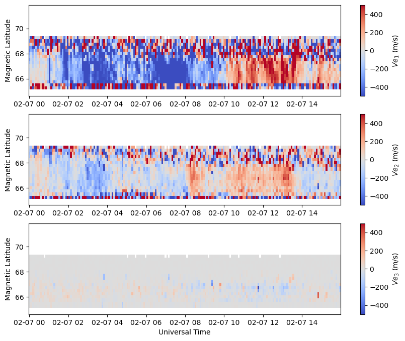
Magnetic Components#
The magnetic components of the velocity vector is the native output of the resolved velocities inversion algorithm. All other output parameters in the file are derived from these.
The plasma drift velocity components \(V_{e_1}\), \(V_{e_2}\), and \(V_{e_3}\) are available in the VvelsMagCoords group in the variable Velocity. This array has the dimensions nrecords x nbins x 3.
Because the inversion algorithm assumes the velocity is purely the \(E \times B\) plasma drift velocity that is perpendicular to the magnetic fields, the \(V_{e_3}\) component SHOULD be zero. This is often not the case in the output, but it is typically orders of magnitude less than the perp-B components and can be thought of as a residual to the fit.
with h5py.File(filepath, 'r') as h5:
    mlat = h5['VvelsMagCoords/Latitude'][:]
    vel = h5['VvelsMagCoords/Velocity'][:]
    utime = h5['Time/UnixTime'][:,0]

time = utime.astype('datetime64[s]')

fig = plt.figure(figsize=(10,8))
gs = gridspec.GridSpec(3,1)
ax = [fig.add_subplot(gs[i]) for i in range(3)]
for i in range(3):
    c = ax[i].pcolormesh(time, mlat, vel[:,:,i].T, vmin=-500., vmax=500., cmap='coolwarm')
    ax[i].set_ylabel('Magnetic Latitude')
    fig.colorbar(c, label=fr'$Ve_{i+1}$ (m/s)')

ax[2].set_xlabel('Universal Time')
Text(0.5, 0, 'Universal Time')
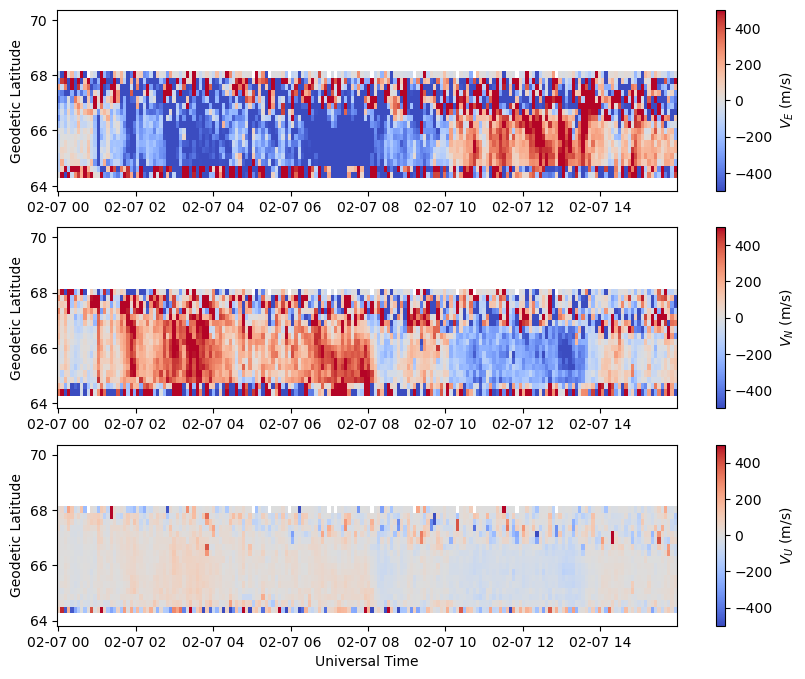
Geodetic Components#
The Geodetic East, North, and Up components of the vector velocities are available in the VvelsGeoCoords group in the variable Velocity. The shape of this array is nrecords x nalt x nbins x 3, where the last dimension is for each of the three E, N, U components respectively. Unlike the magnetic components, the geodetic components DO change in altitude, hence the additional altitude dimension in this array. The values of these altitude slices are in Altitude.
targalt = 300.

with h5py.File(filepath, 'r') as h5:
    alt = h5['VvelsGeoCoords/Altitude'][:,0]
    aidx = np.argmin(np.abs(alt-targalt))
    glat = h5['VvelsGeoCoords/Latitude'][aidx,:]
    vel = h5['VvelsGeoCoords/Velocity'][:,aidx,:,:]
    utime = h5['Time/UnixTime'][:,0]

time = utime.astype('datetime64[s]')

fig = plt.figure(figsize=(10,8))
gs = gridspec.GridSpec(3,1)
ax = [fig.add_subplot(gs[i]) for i in range(3)]
for i, comp in enumerate(['E','N','U']):
    c = ax[i].pcolormesh(time, glat, vel[:,:,i].T, vmin=-500., vmax=500., cmap='coolwarm')
    ax[i].set_ylabel('Geodetic Latitude')
    fig.colorbar(c, label=fr'$V_{comp}$ (m/s)')

ax[2].set_xlabel('Universal Time')
Text(0.5, 0, 'Universal Time')
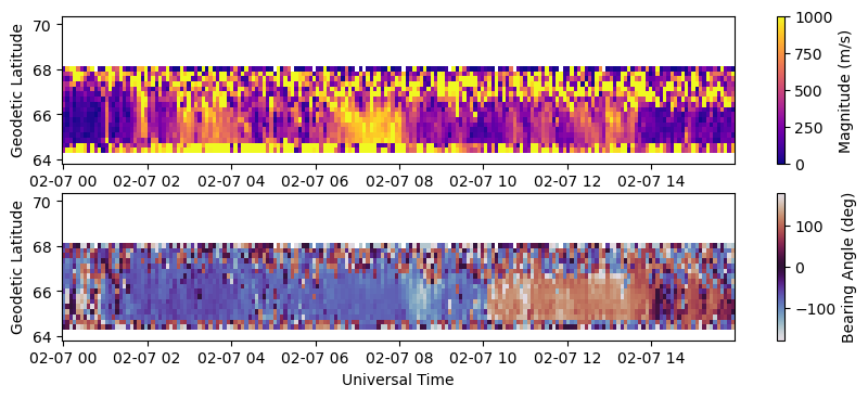
Magnitude and Direction#
The magnitude and horizontal direction (azimuth angle in degrees East of North) of the resolved velocity vectors are also available in the VvelsGeoCoords group as Vmag and Vdir, respectively. These are scalar quantities but also depend on altitude, so have the dimensions nrecords x nalt x nbins.
targalt = 300.

with h5py.File(filepath, 'r') as h5:
    alt = h5['VvelsGeoCoords/Altitude'][:,0]
    aidx = np.argmin(np.abs(alt-targalt))
    glat = h5['VvelsGeoCoords/Latitude'][aidx,:]
    vmag = h5['VvelsGeoCoords/Vmag'][:,aidx,:]
    vdir = h5['VvelsGeoCoords/Vdir'][:,aidx,:]
    utime = h5['Time/UnixTime'][:,0]

time = utime.astype('datetime64[s]')

fig = plt.figure(figsize=(10,6))
gs = gridspec.GridSpec(3,1)
ax = fig.add_subplot(gs[0])
c = ax.pcolormesh(time, glat, vmag.T, vmin=0., vmax=1000., cmap='plasma')
ax.set_ylabel('Geodetic Latitude')
fig.colorbar(c, label='Magnitude (m/s)')

ax = fig.add_subplot(gs[1])
c = ax.pcolormesh(time, glat, vdir.T, vmin=-180., vmax=180., cmap='twilight')
ax.set_xlabel('Universal Time')
ax.set_ylabel('Geodetic Latitude')
fig.colorbar(c, label='Bearing Angle (deg)')
<matplotlib.colorbar.Colorbar at 0x131483100>
Electric Field#
The electric field is calculated from the vector velocity, assuming only \(E \times B\) plasma drift.
The electric field and velocity in the resolved velocities files are not independent measurements. Both are provided for user convenience. By definition, there is no parallel electric field component (\(E_{d_3} = 0 \)).
Similar to velocity, the output files contain the electric field in both geodetic and magnetic coordinates stored in the VvelsGeoCoords and the VvelsMagCoords groups respectively.
Magnetic Components#
The electric field components \(E_{d_1}\), \(E_{d_2}\), and \(E_{d_3}\) are available in the VvelsMagCoords group in the variable Electric Field. This array has the dimensions nrecords x nbins x 3.
with h5py.File(filepath, 'r') as h5:
    mlat = h5['VvelsMagCoords/Latitude'][:]
    efield = h5['VvelsMagCoords/ElectricField'][:]
    utime = h5['Time/UnixTime'][:,0]

time = utime.astype('datetime64[s]')

fig = plt.figure(figsize=(10,8))
gs = gridspec.GridSpec(3,1)
ax = [fig.add_subplot(gs[i]) for i in range(3)]
for i in range(3):
    c = ax[i].pcolormesh(time, mlat, efield[:,:,i].T, vmin=-0.05, vmax=0.05, cmap='coolwarm')
    ax[i].set_ylabel('Magnetic Latitude')
    fig.colorbar(c, label=fr'$Ed_{i+1}$ (V/m)')

ax[2].set_xlabel('Universal Time')
Text(0.5, 0, 'Universal Time')
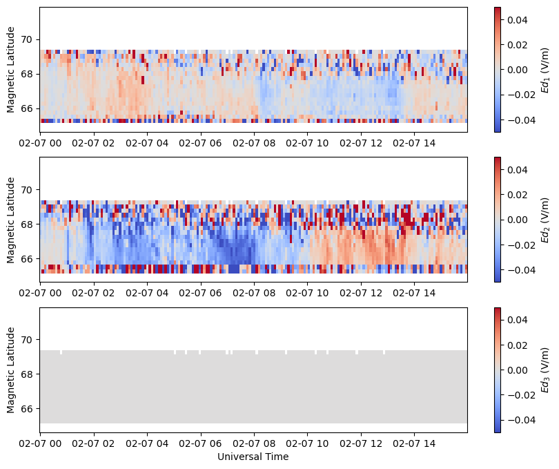
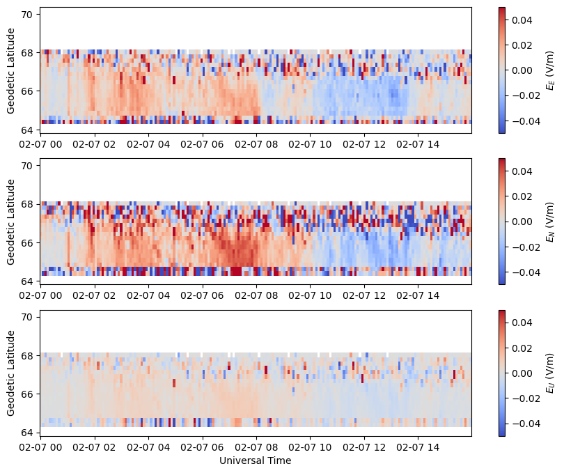
Geodetic Components#
The Geodetic East, North, and Up components of the electric field are available in the VvelsGeoCoords group in the variable ElectricField. The shape of this array is nrecords x nalt x nbins x 3, where the last dimension is for each of the three E, N, U components respectively. Similar to the velocity, the additional altitude dimension captures the fact that the geodetic components change in altitude and the value of each altitude slice can be found in Altitude.
targalt = 300.

with h5py.File(filepath, 'r') as h5:
    alt = h5['VvelsGeoCoords/Altitude'][:,0]
    aidx = np.argmin(np.abs(alt-targalt))
    glat = h5['VvelsGeoCoords/Latitude'][aidx,:]
    efield = h5['VvelsGeoCoords/ElectricField'][:,aidx,:,:]
    utime = h5['Time/UnixTime'][:,0]

time = utime.astype('datetime64[s]')

fig = plt.figure(figsize=(10,8))
gs = gridspec.GridSpec(3,1)
ax = [fig.add_subplot(gs[i]) for i in range(3)]
for i, comp in enumerate(['E','N','U']):
    c = ax[i].pcolormesh(time, glat, efield[:,:,i].T, vmin=-0.05, vmax=0.05, cmap='coolwarm')
    ax[i].set_ylabel('Geodetic Latitude')
    fig.colorbar(c, label=fr'$E_{comp}$ (V/m)')

ax[2].set_xlabel('Universal Time')
Text(0.5, 0, 'Universal Time')
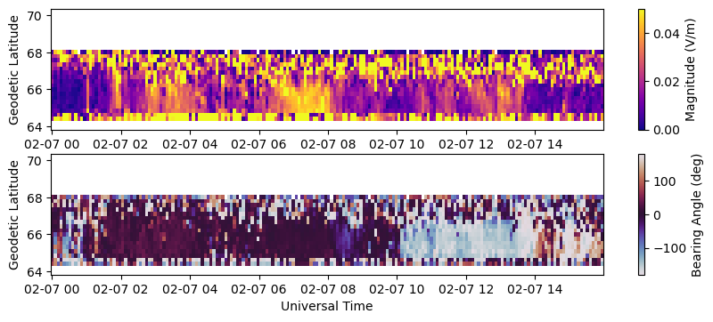
Magnitude and Direction#
The magnitude and horizontal direction (azimuth angle in degrees East of North) of the electric field are also available in the VvelsGeoCoords group as Emag and Edir, respectively. These are scalar quantities but also depend on altitude, so have the dimensions nrecords x nalt x nbins.
targalt = 300.

with h5py.File(filepath, 'r') as h5:
    print(h5['VvelsGeoCoords'].keys())
    alt = h5['VvelsGeoCoords/Altitude'][:,0]
    aidx = np.argmin(np.abs(alt-targalt))
    glat = h5['VvelsGeoCoords/Latitude'][aidx,:]
    emag = h5['VvelsGeoCoords/Emag'][:,aidx,:]
    edir = h5['VvelsGeoCoords/Edir'][:,aidx,:]
    utime = h5['Time/UnixTime'][:,0]

time = utime.astype('datetime64[s]')

fig = plt.figure(figsize=(10,6))
gs = gridspec.GridSpec(3,1)
ax = fig.add_subplot(gs[0])
c = ax.pcolormesh(time, glat, emag.T, vmin=0., vmax=0.05, cmap='plasma')
ax.set_ylabel('Geodetic Latitude')
fig.colorbar(c, label='Magnitude (V/m)')

ax = fig.add_subplot(gs[1])
c = ax.pcolormesh(time, glat, edir.T, vmin=-180., vmax=180., cmap='twilight')
ax.set_xlabel('Universal Time')
ax.set_ylabel('Geodetic Latitude')
fig.colorbar(c, label='Bearing Angle (deg)')
<KeysViewHDF5 ['Altitude', 'CovarianceE', 'CovarianceV', 'Edir', 'ElectricField', 'Emag', 'Latitude', 'Longitude', 'Vdir', 'Velocity', 'Vmag', 'errEdir', 'errElectricField', 'errEmag', 'errVdir', 'errVelocity', 'errVmag']>
<matplotlib.colorbar.Colorbar at 0x12abc78e0>
Convert Magnetic to Geodetic#
To convert magnetic vector components to geodetic vector components, use apexpy to find the base vectors for that location. Then use Laundal and Richmond, 2017 eqn 75/77 to calculate the geodetic components of the vector.
When converting arrays of velocity vectors, it can be helpful to use Einstein notation with numpy.einsum.
For most use cases, geodetic components can be found in the VvelsGeoCoords, where they have been pre-calculated at set altitudes for user convenience. Users should only have to manually convert from apex components to geodetic when velocity at a very specific altitude is needed, or other unusual circumstances.
with h5py.File(filepath, 'r') as h5:
    print(h5['VvelsMagCoords'].keys())
    mlat = h5['VvelsMagCoords/Latitude'][:]
    mlon = h5['VvelsMagCoords/Longitude'][:]
    vel = h5['VvelsMagCoords/Velocity'][:]
    efield = h5['VvelsMagCoords/ElectricField'][:]

A = Apex(2020)

# Convert a single point with a target altitude of 300 km
targalt = 300.
tidx = 10
bidx = 5
f1, f2, f3, g1, g2, g3, d1, d2, d3, e1, e2, e3 = A.basevectors_apex(mlat[bidx], mlon[bidx], targalt, coords='apex')
Ve1, Ve2, Ve3 = vel[tidx,bidx,:]
Ed1, Ed2, Ed3 = efield[tidx,bidx,:]

Vgeo = Ve1*e1 + Ve2*e2
print(f'Geodetic Velocity Components: {Vgeo}')
Egeo = Ed1*d1 + Ed2*d2
print(f'Geodetic Electric Field Components: {Egeo}')

# Convert full array
f1, f2, f3, g1, g2, g3, d1, d2, d3, e1, e2, e3 = A.basevectors_apex(mlat, mlon, 300., coords='apex')
e = np.array([e1, e2]).transpose((2,0,1))
d = np.array([d1, d2]).transpose((2,0,1))

Vgeo = np.einsum('...ij,ijk->...ik',vel[:,:,:2],e)
print(f'Original Velocity Shape: {vel.shape}')
print(f'Converted Velocity Shape: {Vgeo.shape}')

Egeo = np.einsum('...ij,ijk->...ik',efield[:,:,:2],d)
print(f'Original Electric Field Shape: {efield.shape}')
print(f'Converted Electric Field Shape: {Egeo.shape}')
<KeysViewHDF5 ['CovarianceE', 'CovarianceV', 'ElectricField', 'Latitude', 'Longitude', 'Velocity', 'errElectricField', 'errVelocity']>
Geodetic Velocity Components: [-55.96753607 -34.19414676 -11.09833093]
Geodetic Electric Field Components: [-0.00176155  0.00272533  0.0004865 ]
Original Velocity Shape: (188, 29, 3)
Converted Velocity Shape: (188, 29, 3)
Original Electric Field Shape: (188, 29, 3)
Converted Electric Field Shape: (188, 29, 3)
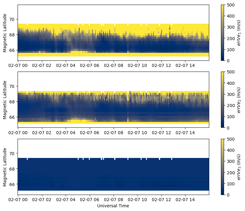
Vector Errors#
The resolved velocities files contain error arrays for the components (geodetic and magnetic), magnitudes, and directions. The files also contain the full covariance matrices for the component arrays. These are nessisary for error propogation when converting between different coordinate systems and other vector calculations. The magnetic component covariance matrices have the shape nrecords x nbins x 3 x 3 while the geodetic component covariance matrices have the shape nrecords x nalt x nbins x 3 x 3. The additional dimension in both cases represents the fact that the covariance matrix for a vector of length 3 has the shape 3 x 3. To calculate the errors on individual components from a covariance matrix, take the square root of the diagonal components.
Plotting the error arrays reveals that the errors get extremely high in the northern-most and southern-most magnetic latitude bins where there are often few points in each bin to control the inversion. This corresponds to the regions in the above plots that show a great deal of “salt and pepper” noise, and should generally not be trusted.
with h5py.File(filepath, 'r') as h5:
    mlat = h5['VvelsMagCoords/Latitude'][:]
    mlon = h5['VvelsMagCoords/Longitude'][:]
    vel = h5['VvelsMagCoords/Velocity'][:]
    errv = h5['VvelsMagCoords/errVelocity'][:]
    covv = h5['VvelsMagCoords/CovarianceV'][:]
    efield = h5['VvelsMagCoords/ElectricField'][:]
    erre = h5['VvelsMagCoords/errElectricField'][:]
    cove = h5['VvelsMagCoords/CovarianceE'][:]
    utime = h5['Time/UnixTime'][:,0]

time = utime.astype('datetime64[s]')

print(f'Velocity Shape: {vel.shape}')
print(f'Velocity Error Shape: {errv.shape}')
print(f'Velocity Covariance Shape: {covv.shape}')

print(f'Electric Field Shape: {efield.shape}')
print(f'Electric Field Error Shape: {erre.shape}')
print(f'Electric Field Covariance Shape: {cove.shape}')

fig = plt.figure(figsize=(10,8))
gs = gridspec.GridSpec(3,1)
ax = [fig.add_subplot(gs[i]) for i in range(3)]
for i in range(3):
    c = ax[i].pcolormesh(time, mlat, errv[:,:,i].T, vmin=0., vmax=500., cmap='cividis')
    ax[i].set_ylabel('Magnetic Latitude')
    fig.colorbar(c, label=fr'$err Ve_{i+1}$ (m/s)')

ax[2].set_xlabel('Universal Time')
Velocity Shape: (188, 29, 3)
Velocity Error Shape: (188, 29, 3)
Velocity Covariance Shape: (188, 29, 3, 3)
Electric Field Shape: (188, 29, 3)
Electric Field Error Shape: (188, 29, 3)
Electric Field Covariance Shape: (188, 29, 3, 3)
Text(0.5, 0, 'Universal Time')
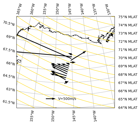
Plot Vectors on Map#
To create a map of the velocity or electric field vectors on a map, load the geodetic components of the quantity of interest an plot them with quiver and cartopy. Only the geodetic East and geodetic North components can be displayed this way.
targalt = 300.
utargtime = np.datetime64('2020-02-07T07:00:00', '[s]').astype(int)

with h5py.File(filepath, 'r') as h5:

    site_lat = h5['Site/Latitude'][()]
    site_lon = h5['Site/Longitude'][()]
    alt = h5['VvelsGeoCoords/Altitude'][:,0]
    aidx = np.argmin(np.abs(alt-targalt))
    utime = h5['Time/UnixTime'][:,0]
    tidx = np.argmin(np.abs(utargtime-utime))
    glat = h5['VvelsGeoCoords/Latitude'][aidx,:]
    glon = h5['VvelsGeoCoords/Longitude'][aidx,:]
    vel = h5['VvelsGeoCoords/Velocity'][tidx,aidx,:,:]

time = utime.astype('datetime64[s]')

# generate figure
fig = plt.figure()

# create map
proj = ccrs.AzimuthalEquidistant(central_longitude=site_lon, central_latitude=site_lat)
ax = fig.add_subplot(111, projection=proj)
gl = ax.gridlines(draw_labels=True, zorder=1)
gl.right_labels = False
ax.coastlines()
ax.set_extent([-159., -135., 61., 72.], crs=ccrs.PlateCarree())

# This function is needed due to an issue with cartopy where vectors are not scale/rotated
#   correctly in some coordinate systems (see: https://github.com/SciTools/cartopy/issues/1179)
def scale_uv(lon, lat, u, v):
    us = u/np.cos(lat*np.pi/180.)
    vs = v
    sf = np.sqrt(u**2+v**2)/np.sqrt(us**2+vs**2)
    return us*sf, vs*sf

u, v = scale_uv(glon, glat, vel[:,0], vel[:,1])
Q = ax.quiver(glon, glat, u, v, zorder=5, scale=5000, linewidth=2, color='k', transform=ccrs.PlateCarree())

ax.quiverkey(Q, 0.4, 0.1, 500, 'V=500m/s', labelpos='E', transform=ax.transAxes)


# Add magnetic parallels for visualization convenience
mlon_arr = np.linspace(-150., -50., 100)
x0, x1, y0, y1 = ax.get_extent()

for mlat in np.arange(60., 76., 1.):
    mlat_arr = np.full(100, mlat)

    glat_arr, glon_arr, _ = A.apex2geo(mlat_arr, mlon_arr, height=targalt)
    line = proj.transform_points(ccrs.Geodetic(), glon_arr, glat_arr)
    ax.plot(line[:,0], line[:,1], linewidth=1., color='gold', zorder=2)

    yl = np.interp(x1, line[:,0], line[:,1])
    if yl>y0 and yl<y1:
        ax.text(x1+5e4, yl, f'{mlat:.0f}°N MLAT', verticalalignment='center')